Last week at the Splunk user conference in San Francisco, Paul Sanford from the Splunk SDK team demoed a solution we helped assemble showing easy SQL access to data in Splunk. It was very well received and we look forward to helping Splunk users access their data via SQL and commodity BI tools!
While you won’t find it in their marketing materials, Splunk is a battle hardened, production grade NoSQL system (at least for analytics). They have a massively scalable, distributed compute engine (ie, Map-Reduce-eee) along with free form schema-less type data processing. So, while they don’t necessarily throw their ring into new NoSQL type projects (and let’s be honest, if you’re not Open Source it’d be hard to get selected for a new project) their thousands of customers have been very happy with their ingestion, alerting, and reporting on IT data and is very NoSQL-eee.
The SDK team has been working on opening up the underlying engine, framework so that additional developers can innovate and do some cool stuff on top of Splunk. Splunk developers from California (some of whom worked at LucidEra prior) kick started a project that gives LucidDB the ability to talk to Splunk hereby enabling SQL access to commodity BI tools. We’ve adopted the project, and built out some examples using Pentaho to show the power of SQL access to Splunk.
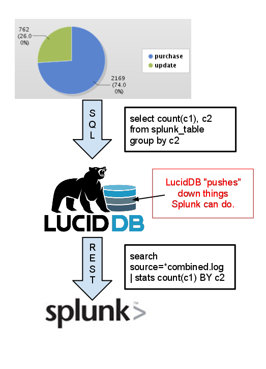
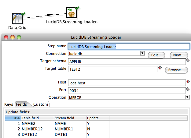
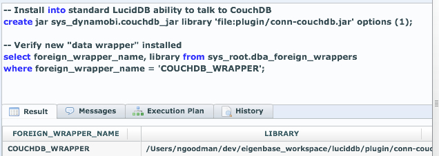
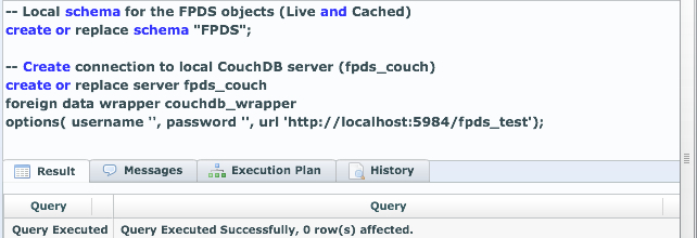
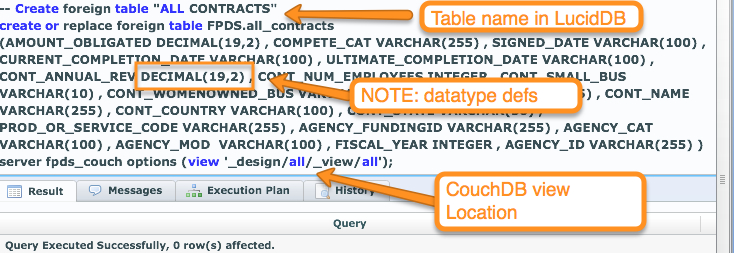
First off, our overall approach is similar to our existing ability to talk to CouchDB, Hive/Hadoop, etc remains the same.
- We learn how to speak the remote language (in this case, Spunk search queries) generally. This means we can simply stream data across the wire in it’s entirety and then do all the SQL
- We enable some rewrite rules so that if the remote system (Splunk) knows how to do things (such as simple filtering in the WHERE clause, or GROUP BY stats) we’ll rewrite our query and push more to the work down to the remote system.
Once we’ve done that, we can enable any BI tool (that can do things such as SQL, read catalogs/tables, enable metadata/etc) connect up and do cool things like drag and drop reports. Here’s some examples created using Pentaho’s Enterprise Edition 4.0 BI Suite (which looks great, btw!):
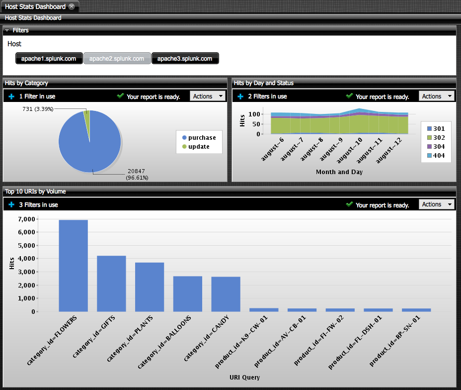
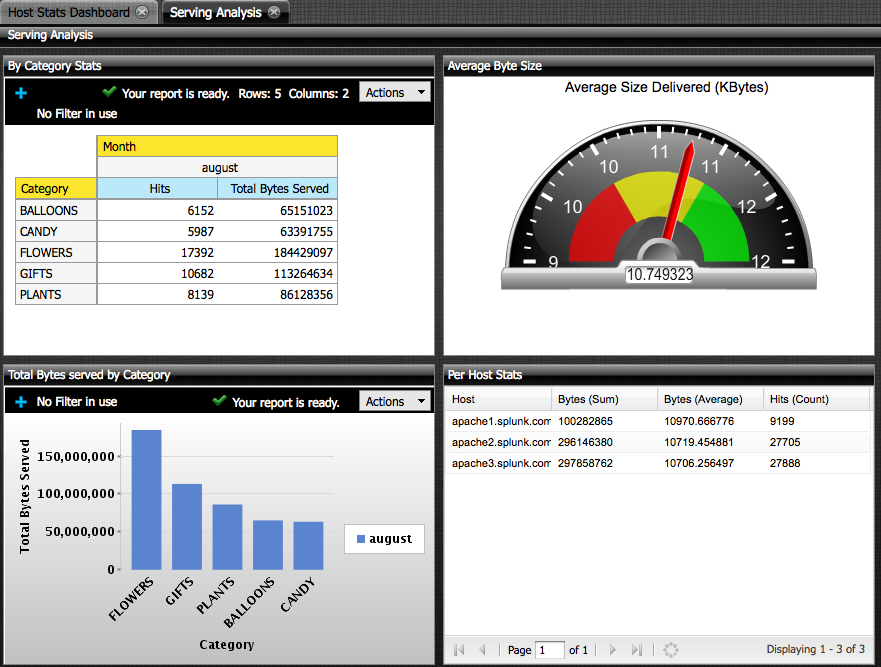
These dashboards were created, entirely within a Web Browser using Drag and Drop (via Pentaho’s modeling/report building capabilities). Total time to build these dashboards was less than 45 minutes including model definition and report building (caveat: I know Pentaho dashboards inside and out).
Splunk users can now access data in their Splunk system, including matching/mashing it with others simply and easily in everyday, inexpensive BI tools.
In fact, this project came about initially as a Splunk customer wanted to do some advanced visualization in Tableau. Using our experimental ODBC Connectivity the user was able to visualize their Splunk data in Tableau using some of their fantastic visualizations.